R lecture 2: R basics

SKI3011 · objects, vectors, data frames, reading data, data types, plots

How to use this lecture. Download the R script, open it in RStudio and run it line by line (Cmd+Enter on a Mac, Ctrl+Enter on Windows). All explanations on this page are in the script as comments. Check that you get the same output as shown here. Quiz 1 asks you to read and interpret exactly this kind of code and output.

Download the R script Download the practice file bcg.csv

Why R?

R is a program for statistical computing, not just for meta-analyses. To learn to do a meta-analysis in R, we first need the basics. A general principle of responsible research: keep only two files, the raw data file and the script. Never change the raw data by hand without logging it: every change is a line in the script.

R as a calculator

4 + 3

[1] 7

4 * 2

[1] 8

4^2

[1] 16

log(4)    # natural logarithm

[1] 1.386294

exp(4)    # the inverse of log()

[1] 54.59815

sqrt(4)

[1] 2

Vectors and functions

A vector combines values that belong together, like a column in a spreadsheet: the ages of participants, or the effect sizes of the studies in a meta-analysis. c() stands for combine. A function such as mean() takes arguments between brackets. Use ? to open the help page of a function.

c(9, 3, 6)

[1] 9 3 6

mean(c(9, 3, 6))

[1] 6

sd(c(9, 3, 6))

[1] 3

sort(c(9, 3, 6), decreasing = TRUE)   # an extra argument changes what the function does

[1] 9 6 3

# ?sort                               # remove the # to open the help page

Objects

A vector, a dataset or a single value can be stored in an object with <-. You choose the name yourself. The object appears in the Environment window (top right in RStudio).

a <- c(9, 3, 6)
a

[1] 9 3 6

b <- 2 + 2
a / b      # every value of a is divided by b

[1] 2.25 0.75 1.50

z <- a / b
z

[1] 2.25 0.75 1.50

Data frames

A data frame is a table: one row per study, one column per variable. Here we make the meta-analysis dataset you know from SKI3010 by hand: 11 studies on environmental tobacco smoke at home and bladder cancer, with the log odds ratio and its standard error.

lnOR <- c(-0.223143551, -0.198450939, -0.162518929, -0.162518929, -0.116533816, 0.009950331,
          0.086177696, 0.139761942, 0.165514438, 0.336472237, 0.457424847)
se <- c(0.38457745, 0.301271952, 0.200831965, 0.279480271, 0.359347184, 0.428673775,
        0.247347883, 0.162072911, 0.251023247, 0.3350916, 0.293754916)
firstauthor <- c("Alberg (2)", "Bjerregaard", "Jiang", "Burch", "NLCS", "Kabat",
                 "Baris", "Zheng", "Samanic", "Alberg (1)", "Tao")
year <- c(2007, 2006, 2007, 1989, 2002, 1986, 2009, 2012, 2006, 2007, 2010)
dat <- data.frame(firstauthor, year, lnOR, se)
dat

   firstauthor year         lnOR        se
1   Alberg (2) 2007 -0.223143551 0.3845774
2  Bjerregaard 2006 -0.198450939 0.3012720
3        Jiang 2007 -0.162518929 0.2008320
4        Burch 1989 -0.162518929 0.2794803
5         NLCS 2002 -0.116533816 0.3593472
6        Kabat 1986  0.009950331 0.4286738
7        Baris 2009  0.086177696 0.2473479
8        Zheng 2012  0.139761942 0.1620729
9      Samanic 2006  0.165514438 0.2510232
10  Alberg (1) 2007  0.336472237 0.3350916
11         Tao 2010  0.457424847 0.2937549

names(dat)                # the column names

[1] "firstauthor" "year"        "lnOR"        "se"         

dat$lnOR                  # $ selects one column

 [1] -0.223143551 -0.198450939 -0.162518929 -0.162518929 -0.116533816
 [6]  0.009950331  0.086177696  0.139761942  0.165514438  0.336472237
[11]  0.457424847

dat$year[2]               # [ ] selects an element: the second year

[1] 2006

dat[dat$year > 2006, ]    # the rows of studies published after 2006

   firstauthor year       lnOR        se
1   Alberg (2) 2007 -0.2231436 0.3845774
3        Jiang 2007 -0.1625189 0.2008320
7        Baris 2009  0.0861777 0.2473479
8        Zheng 2012  0.1397619 0.1620729
10  Alberg (1) 2007  0.3364722 0.3350916
11         Tao 2010  0.4574248 0.2937549

round(exp(dat$lnOR), 2)   # back from log odds ratios to odds ratios

 [1] 0.80 0.82 0.85 0.85 0.89 1.01 1.09 1.15 1.18 1.40 1.58

# View(dat)               # opens the data in a spreadsheet view

Reading a csv file

Most of your data will come from a spreadsheet saved as csv. Download the practice file bcg.csv and put it in the folder where you keep your script. getwd() shows the folder R works in; in RStudio you can change it via Session, Set Working Directory, To Source File Location.

European csv files use a semicolon as separator and a comma as decimal sign. If you forget that, R reads everything into one column:

# getwd()                    # which folder is R working in?
wrong <- read.csv("bcg.csv")
head(wrong, 2)               # one column, everything glued together

                                        author.year.tpos.tneg.cpos.cneg.ablat.risk_vaccinated
Aronson;1948;4;119;11;128;44;0                                                            325
Ferguson & Simes;1949;6;300;29;274;55;0                                                   196

Tell R which separator and decimal sign the file uses:

bcg <- read.csv("bcg.csv", sep = ";", dec = ",")
head(bcg, 3)

            author year tpos tneg cpos cneg ablat risk_vaccinated
1          Aronson 1948    4  119   11  128    44          0.0325
2 Ferguson & Simes 1949    6  300   29  274    55          0.0196
3  Rosenthal et al 1960    3  228   11  209    42          0.0130

dim(bcg)        # number of rows (studies) and columns (variables)

[1] 13  8

Data types

R distinguishes numeric values (for calculations), logical values (TRUE or FALSE), character values (text) and factors (categories). class() tells you which type an object is.

a <- 44 / 5
class(a)

[1] "numeric"

b <- 7 > 4
b

[1] TRUE

class(b)

[1] "logical"

class(bcg$author)

[1] "character"

pets <- c("cat", "dog", "cat", "bird", "cat")
class(pets)

[1] "character"

pets <- as.factor(pets)   # a factor: a categorical variable with levels
levels(pets)

[1] "bird" "cat"  "dog" 

Some simple statistics

R has built-in datasets. airquality contains daily air measurements in New York. Does ozone concentration depend on temperature? In lm() the tilde ~ separates the outcome from the explanatory variable.

dim(airquality)

[1] 153   6

head(airquality, 3)

  Ozone Solar.R Wind Temp Month Day
1    41     190  7.4   67     5   1
2    36     118  8.0   72     5   2
3    12     149 12.6   74     5   3

fit <- lm(Ozone ~ Temp, data = airquality)
summary(fit)

Call:
lm(formula = Ozone ~ Temp, data = airquality)

Residuals:
    Min      1Q  Median      3Q     Max 
-40.729 -17.409  -0.587  11.306 118.271 

Coefficients:
             Estimate Std. Error t value Pr(>|t|)    
(Intercept) -146.9955    18.2872  -8.038 9.37e-13 ***
Temp           2.4287     0.2331  10.418  < 2e-16 ***
---
Signif. codes:  0 '***' 0.001 '**' 0.01 '*' 0.05 '.' 0.1 ' ' 1

Residual standard error: 23.71 on 114 degrees of freedom
  (37 observations deleted due to missingness)
Multiple R-squared:  0.4877,    Adjusted R-squared:  0.4832 
F-statistic: 108.5 on 1 and 114 DF,  p-value: < 2.2e-16

Plots

The built-in dataset iris has flower measurements of three species. Arguments such as main, xlab, pch and col change the title, axis labels, symbols and colours.

hist(iris$Petal.Length, main = "Histogram of petal length", xlab = "Petal length")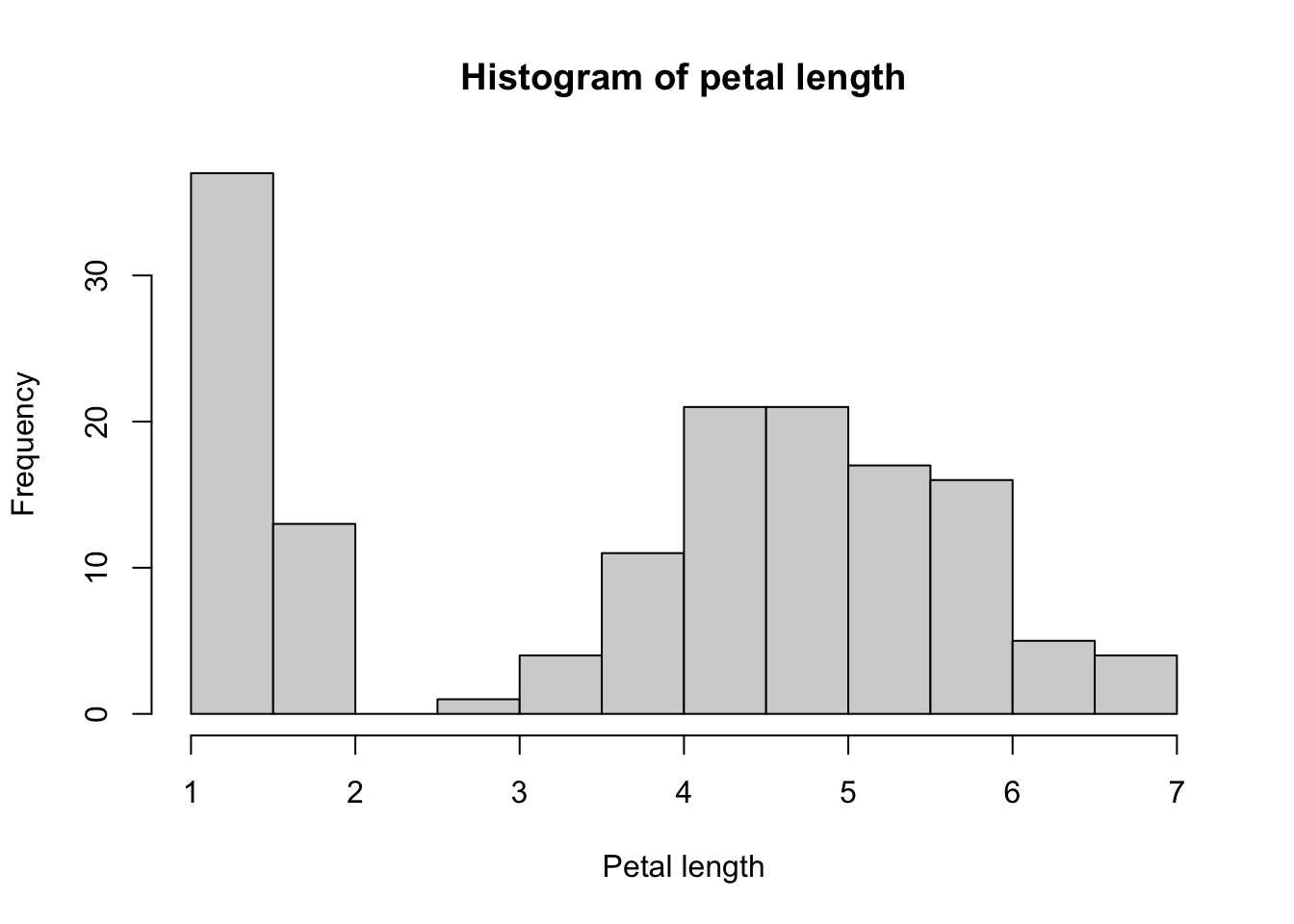

boxplot(Petal.Length ~ Species, data = iris,
        main = "Petal length by species", xlab = "Species", ylab = "Petal length")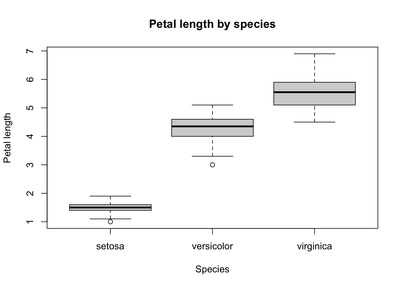

plot(iris$Petal.Length, iris$Sepal.Length, pch = 20, col = "darkorange",
     main = "Petal length and sepal length", xlab = "Petal length", ylab = "Sepal length")
abline(lm(Sepal.Length ~ Petal.Length, data = iris))   # add the regression line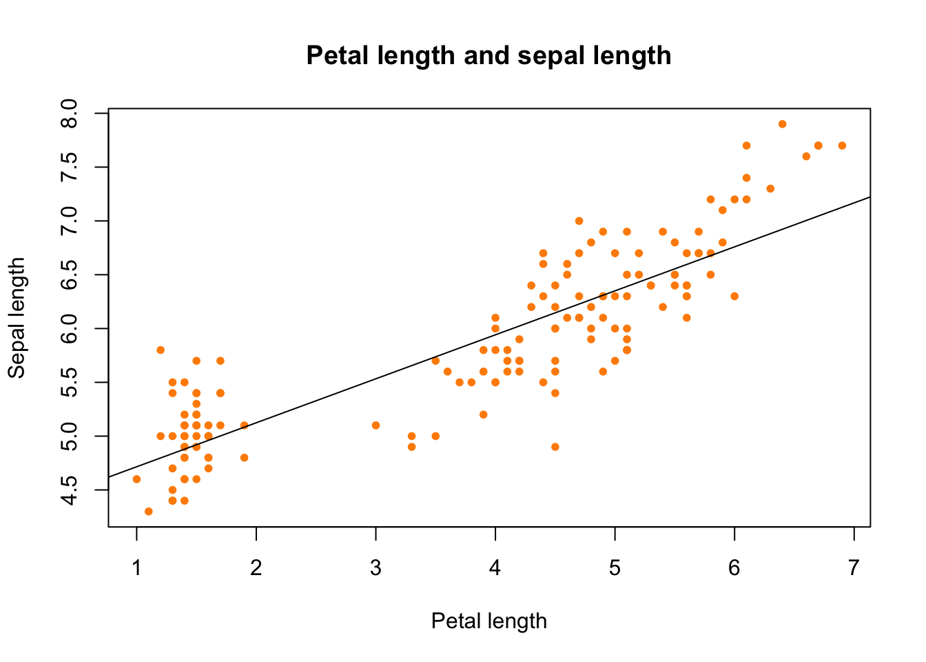

Saving your data

write.csv() saves a data frame as a csv file in your working directory; read.csv() reads it back. This line is not run on the website.

write.csv(bcg, "my_bcg_data.csv", row.names = FALSE)
my_data <- read.csv("my_bcg_data.csv")

Now your own data

Import your own extraction sheet (saved as csv) with read.csv() and check it with head(), dim() and class().

Check yourself

Go to the concept list and practice quiz of week 2 and try the practice quiz without looking at this page.