# install.packages(c("metafor", "metadat"))   # run once, remove the # to run it
library(metafor)   # meta-analysis functions: escalc(), rma(), forest()
library(metadat) # example datasets, such as dat.bcgR lecture 3: Meta-analysis in R I
SKI3011 · escalc(), rma(), forest plots, proportions and correlations
How to use this lecture. Download the R script, open it in RStudio and run it line by line (Cmd+Enter on a Mac, Ctrl+Enter on Windows). All explanations on this page are in the script as comments. Check that you get the same output as shown here. Quiz 2 asks you to read and interpret exactly this kind of code and output.
Packages
install.packages() installs a package once on your computer; library() loads it in every new R session.
The BCG data
13 trials of the BCG vaccine against tuberculosis. tpos and tneg are the TB-positive and TB-negative people in the vaccinated group, cpos and cneg the same in the control group: the four cells of the 2×2 table. ablat is the absolute latitude of the trial site; we use it in week 6.
head(dat.bcg[, c("author", "year", "tpos", "tneg", "cpos", "cneg", "ablat")], 4) author year tpos tneg cpos cneg ablat
1 Aronson 1948 4 119 11 128 44
2 Ferguson & Simes 1949 6 300 29 274 55
3 Rosenthal et al 1960 3 228 11 209 42
4 Hart & Sutherland 1977 62 13536 248 12619 52Step 1: one effect size per study
escalc() adds two columns to the data: yi, the log risk ratio, and vi, its sampling variance (SE²). Ratios are always stored on the log scale.
dat <- escalc(measure = "RR",                              # effect size: risk ratio (also "OR", "RD", "MD", "SMD", "PR", "ZCOR")
              ai = tpos, bi = tneg, ci = cpos, di = cneg,  # the four cells of the 2x2 table
              data = dat.bcg,
              slab = paste(author, year))                  # study labels for the output and the forest plot
head(dat[, c("author", "year", "yi", "vi")], 4)
             author year      yi     vi
1           Aronson 1948 -0.8893 0.3256
2  Ferguson & Simes 1949 -1.5854 0.1946
3   Rosenthal et al 1960 -1.3481 0.4154
4 Hart & Sutherland 1977 -1.4416 0.0200
Step 2: random-effects meta-analysis
rma() fits a random-effects model by default, with τ² estimated by REML. tau^2, I^2 and the Q test describe heterogeneity (week 5). estimate is the pooled log risk ratio: −0.71.
res <- rma(yi, vi, data = dat)   # random-effects model (default method: REML)
print(res, digits = 2)
Random-Effects Model (k = 13; tau^2 estimator: REML)

tau^2 (estimated amount of total heterogeneity): 0.31 (SE = 0.17)
tau (square root of estimated tau^2 value):      0.56
I^2 (total heterogeneity / total variability):   92.22%
H^2 (total variability / sampling variability):  12.86

Test for Heterogeneity:
Q(df = 12) = 152.23, p-val < .01

Model Results:

estimate    se   zval  pval  ci.lb  ci.ub
   -0.71  0.18  -3.97  <.01  -1.07  -0.36  ***

---
Signif. codes:  0 '***' 0.001 '**' 0.01 '*' 0.05 '.' 0.1 ' ' 1
Step 3: back to the risk ratio scale
pred = exp(−0.71) = 0.49: vaccinated people have about half the risk of TB (95% CI 0.34 to 0.70). pi.lb and pi.ub are the 95% prediction interval: the range in which the true effect of a new trial is expected to fall (week 5).
predict(res, transf = exp, digits = 2) # exp() turns the log risk ratio back into a risk ratio
 pred ci.lb ci.ub pi.lb pi.ub
 0.49  0.34  0.70  0.15  1.55
Step 4: forest plot
atransf = exp shows risk ratios on the axis instead of log risk ratios. Box size is the weight of each trial; the diamond is the pooled estimate with its 95% CI.
forest(res, atransf = exp, header = TRUE)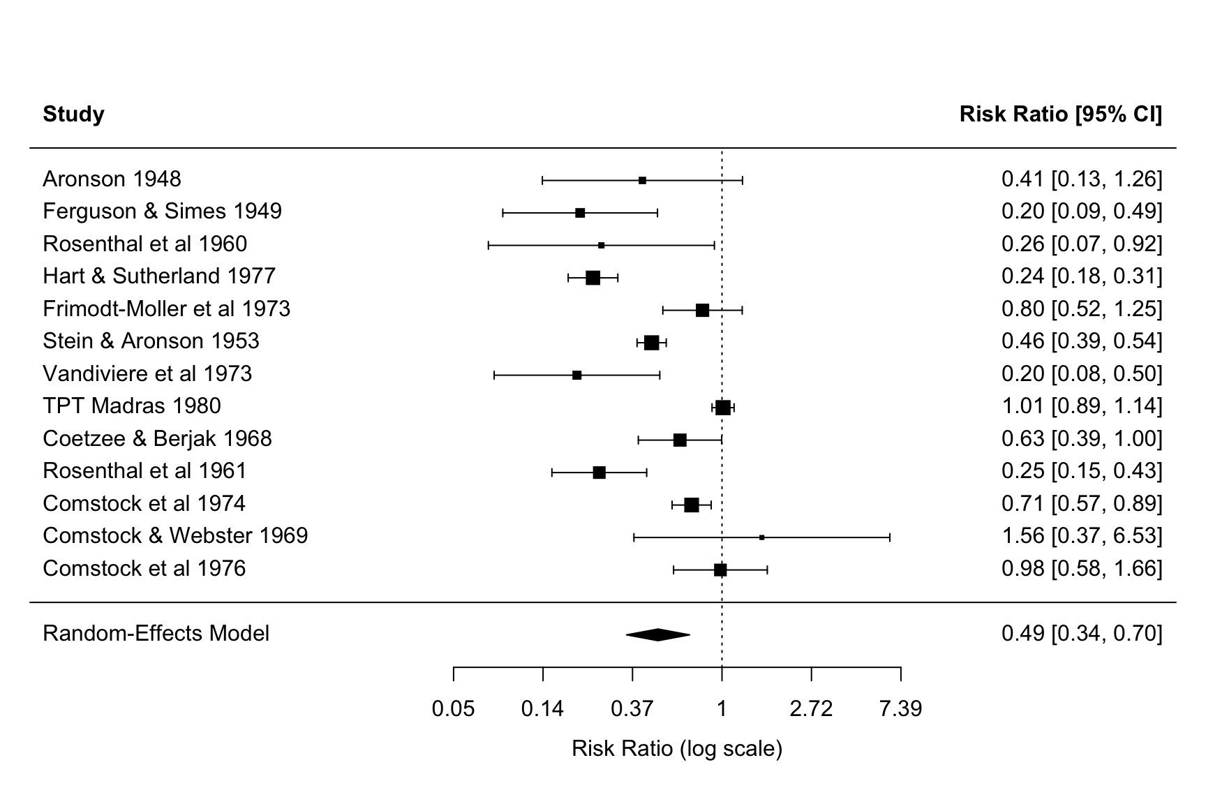
Fixed effect versus random effects
The fixed-effect model assumes one common true effect. Its CI is much narrower (0.60 to 0.70) because it ignores the large between-trial variation: with heterogeneity this big, the random-effects model is the honest choice.
res_fe <- rma(yi, vi, data = dat, method = "FE")   # fixed-effect model
predict(res_fe, transf = exp, digits = 2)
 pred ci.lb ci.ub
 0.65  0.60  0.70
Proportions
35 studies on the proportion of COVID-19 patients with loss of smell (dat.hannum2020). About half of the patients (0.49, 95% CI 0.41 to 0.57) lose their sense of smell. Note the enormous heterogeneity: the studies used objective and subjective measurements (we split them in week 6). For proportions near 0 or 1 a transformation such as "PLO" (logit) is better.
dat_pr <- escalc(measure = "PR", xi = xi, ni = ni, data = dat.hannum2020)   # xi = events, ni = sample size
res_pr <- rma(yi, vi, data = dat_pr)
print(res_pr, digits = 2)
Random-Effects Model (k = 35; tau^2 estimator: REML)

tau^2 (estimated amount of total heterogeneity): 0.06 (SE = 0.01)
tau (square root of estimated tau^2 value):      0.24
I^2 (total heterogeneity / total variability):   99.28%
H^2 (total variability / sampling variability):  138.10

Test for Heterogeneity:
Q(df = 34) = 7878.14, p-val < .01

Model Results:

estimate    se   zval  pval  ci.lb  ci.ub
    0.49  0.04  11.88  <.01   0.41   0.57  ***

---
Signif. codes:  0 '***' 0.001 '**' 0.01 '*' 0.05 '.' 0.1 ' ' 1
Correlations
16 studies on the correlation between conscientiousness and medication adherence (dat.molloy2014). Correlations are pooled after transformation to Fisher’s z and transformed back with transf.ztor. More conscientious patients adhere slightly better to their medication: r = 0.15 (95% CI 0.09 to 0.21). The prediction interval (−0.04 to 0.32) shows that in some settings there may be no association at all.
dat_r <- escalc(measure = "ZCOR", ri = ri, ni = ni, data = dat.molloy2014)   # ri = correlation, ni = sample size
res_r <- rma(yi, vi, data = dat_r)
predict(res_r, transf = transf.ztor, digits = 2)   # back from Fisher's z to a correlation
 pred ci.lb ci.ub pi.lb pi.ub
 0.15  0.09  0.21 -0.04  0.32
Check yourself
Go to the concept list and practice quiz of week 3 and try the practice quiz without looking at this page.