# install.packages("meta")   # run once
library(metafor)
library(meta)
library(metadat)R lecture 4: Meta-analysis in R II
SKI3011 · binary and continuous outcomes, published odds ratios, the meta package
How to use this lecture. Download the R script, open it in RStudio and run it line by line (Cmd+Enter on a Mac, Ctrl+Enter on Windows). All explanations on this page are in the script as comments. Check that you get the same output as shown here. Quiz 3 asks you to read and interpret exactly this kind of code and output.
Packages
Today we use two packages. metafor you know from last week. meta does the same with slightly different functions (metabin(), metacont(), metagen()) and makes nice forest plots. Many published reviews use one of the two.
Binary outcomes: the data
Nine trials on diuretics in pregnancy and the risk of pre-eclampsia (dat.collins1985b). For each trial we need the number of events and the group size in the treatment and the control group.
dat <- dat.collins1985b[, c("author", "year", "pre.xti", "pre.nti", "pre.xci", "pre.nci")]
dat
author year pre.xti pre.nti pre.xci pre.nci
1 Weseley & Douglas 1962 14 131 14 136
2 Flowers et al. 1962 21 385 17 134
3 Menzies 1964 14 57 24 48
4 Fallis et al. 1964 6 38 18 40
5 Cuadros & Tatum 1964 12 1011 35 760
6 Landesman et al. 1965 138 1370 175 1336
7 Kraus et al. 1966 15 506 20 524
8 Tervila & Vartiainen 1971 6 108 2 103
9 Campbell & MacGillivray 1975 65 153 40 102Binary outcomes with metafor
Instead of the four cells (ai, bi, ci, di) you can give the events and group sizes (ai, n1i, ci, n2i). The odds ratio is pooled on the log scale.
dat <- escalc(measure = "OR",
              ai = pre.xti, n1i = pre.nti,   # events and group size, treatment
              ci = pre.xci, n2i = pre.nci,   # events and group size, control
              data = dat, slab = paste(author, year))
res <- rma(yi, vi, data = dat)
predict(res, transf = exp, digits = 2)
 pred ci.lb ci.ub pi.lb pi.ub
 0.60  0.38  0.92  0.19  1.90
Diuretics lower the odds of pre-eclampsia (OR 0.60, 95% CI 0.38 to 0.92), but the prediction interval (0.19 to 1.90) shows that the effect in a new trial could be anything from strong protection to harm: the trials are very heterogeneous.
forest(res, atransf = exp, header = TRUE)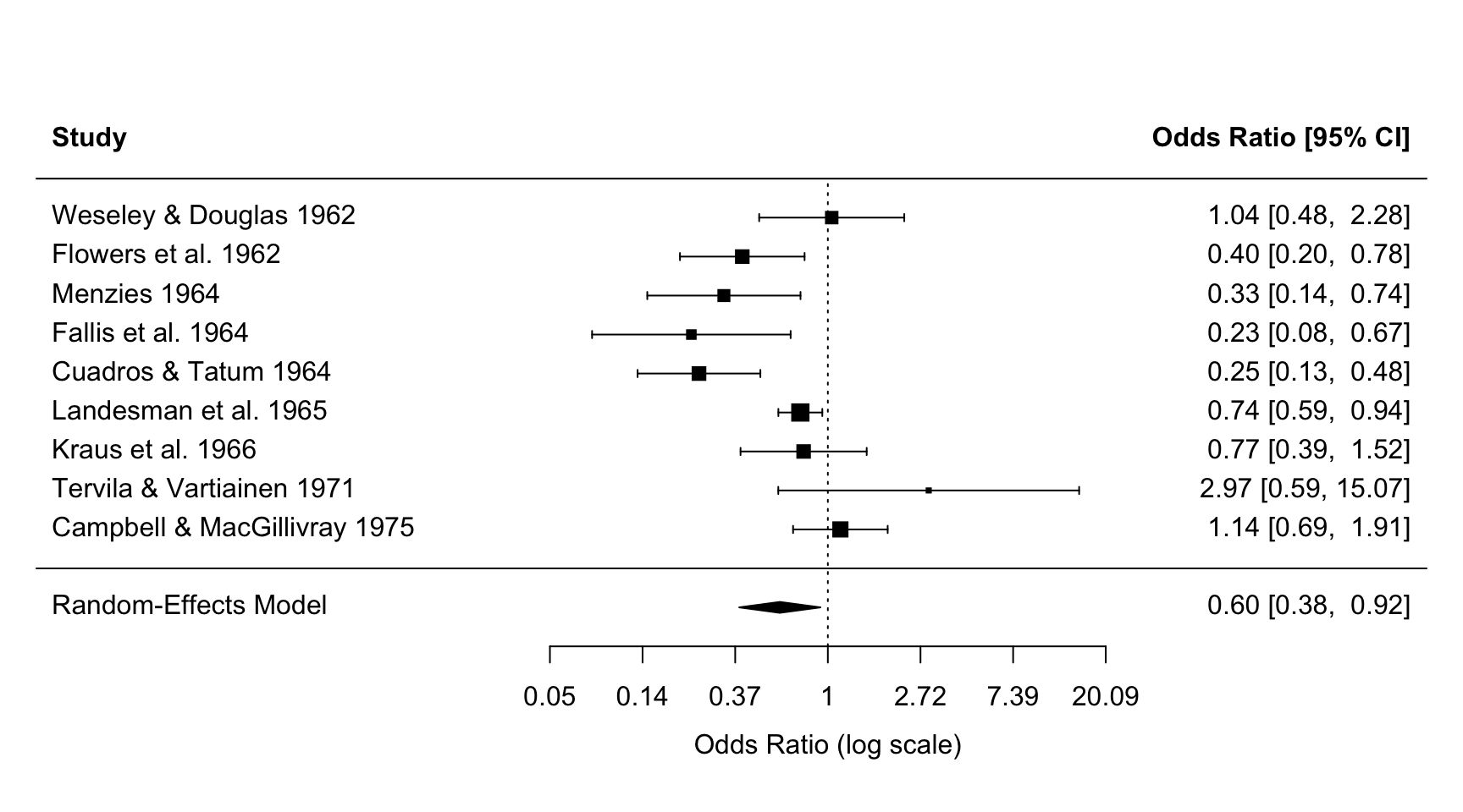
Mantel-Haenszel
The Mantel-Haenszel method is a fixed-effect method that works directly on the counts and handles small numbers of events well.
rma.mh(measure = "OR", ai = pre.xti, n1i = pre.nti, ci = pre.xci, n2i = pre.nci,
       data = dat, digits = 2)
Equal-Effects Model (k = 9)

I^2 (total heterogeneity / total variability):  70.66%
H^2 (total variability / sampling variability): 3.41

Test for Heterogeneity:
Q(df = 8) = 27.27, p-val < .01

Model Results (log scale):

estimate    se   zval  pval  ci.lb  ci.ub
   -0.40  0.09  -4.60  <.01  -0.58  -0.23

Model Results (OR scale):

estimate  ci.lb  ci.ub
    0.67   0.56   0.79

Cochran-Mantel-Haenszel Test:    CMH = 21.23, df = 1, p-val < 0.01
Tarone's Test for Heterogeneity: X^2 = 28.79, df = 8, p-val < 0.01
Binary outcomes with meta
metabin() from the meta package gives the fixed-effect (called “common effect”) and the random-effects result in one go. Studies with zero events in one group get a continuity correction of 0.5 (incr).
m_bin <- metabin(event.e = pre.xti, n.e = pre.nti,   # experimental group
                 event.c = pre.xci, n.c = pre.nci,   # control group
                 sm = "OR", data = dat,
                 studlab = paste(author, year))
summary(m_bin)
OR 95%-CI %W(common) %W(random)
Weseley & Douglas 1962 1.0427 [0.4766; 2.2815] 3.9 10.9
Flowers et al. 1962 0.3971 [0.2027; 0.7779] 7.5 11.9
Menzies 1964 0.3256 [0.1424; 0.7444] 6.2 10.4
Fallis et al. 1964 0.2292 [0.0785; 0.6692] 4.6 8.3
Cuadros & Tatum 1964 0.2488 [0.1283; 0.4827] 12.4 12.0
Landesman et al. 1965 0.7431 [0.5863; 0.9420] 50.1 15.9
Kraus et al. 1966 0.7699 [0.3897; 1.5210] 6.0 11.9
Tervila & Vartiainen 1971 2.9706 [0.5857; 15.0675] 0.6 5.1
Campbell & MacGillivray 1975 1.1449 [0.6871; 1.9078] 8.7 13.6
Number of studies: k = 9
Number of observations: o = 6942 (o.e = 3759, o.c = 3183)
Number of events: e = 636
OR 95%-CI z p-value
Common effect model 0.6677 [0.5620; 0.7932] -4.60 < 0.0001
Random effects model 0.5956 [0.3843; 0.9233] -2.32 0.0205
Quantifying heterogeneity (with 95%-CIs):
tau^2 = 0.3008 [0.0723; 2.2027]; tau = 0.5484 [0.2689; 1.4842]
I^2 = 70.7% [41.8%; 85.2%]; H = 1.85 [1.31; 2.60]
Test of heterogeneity:
Q d.f. p-value
27.26 8 0.0006
Details of meta-analysis methods:
- Mantel-Haenszel method (common effect model)
- Inverse variance method (random effects model)
- Restricted maximum-likelihood estimator for tau^2
- Q-Profile method for confidence interval of tau^2 and tau
- Calculation of I^2 based on Qforest(m_bin)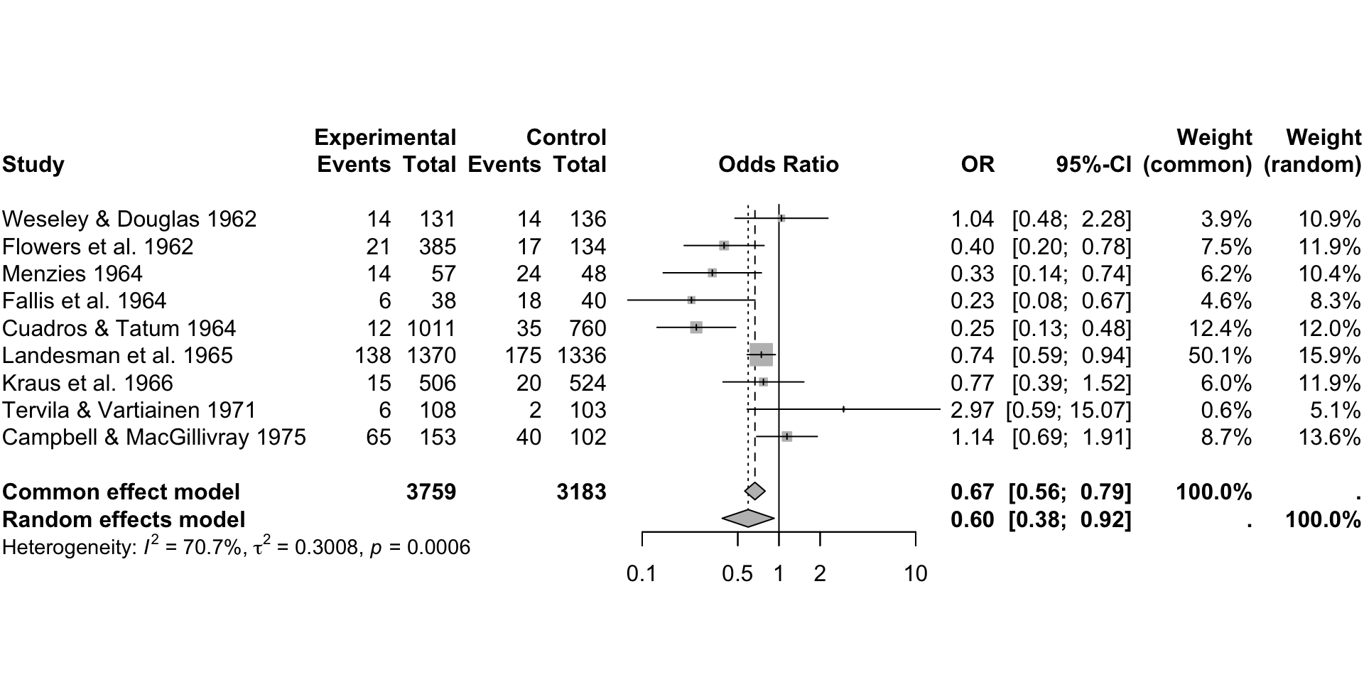
Published odds ratios with a confidence interval
Often a paper only reports an odds ratio with its 95% CI. Then you calculate the log odds ratio and its standard error yourself: SE = [ln(upper) − ln(lower)] / 3.92. Example: 37 studies on passive smoking and lung cancer in women (dat.hackshaw1998).
smoke <- dat.hackshaw1998[, c("author", "year", "or", "or.lb", "or.ub")]
smoke$log_or <- log(smoke$or)
smoke$se_log_or <- (log(smoke$or.ub) - log(smoke$or.lb)) / 3.92   # SE from the 95% CI
head(smoke, 3)
     author year   or or.lb or.ub    log_or se_log_or
1 Garfinkel 1981 1.18  0.90  1.54 0.1655144 0.1370263
2  Hirayama 1984 1.45  1.02  2.08 0.3715636 0.1817769
3    Butler 1988 2.02  0.48  8.56 0.7030975 0.7349667
metagen() pools any pre-calculated effect size: TE is the effect (here the log OR) and seTE its standard error. With sm = "OR" the output is shown as odds ratios.
m_gen <- metagen(TE = log_or, seTE = se_log_or, sm = "OR",
                 data = smoke, studlab = paste(author, year))
summary(m_gen)$random    # random-effects result on the log scale
$TE
[1] 0.2188913
$seTE
[1] 0.04939564
$lower
[1] 0.1220777
$upper
[1] 0.315705
$statistic
[1] 4.43139
$p
[1] 9.36276e-06
$level
[1] 0.95
$df
[1] Infexp(c(m_gen$TE.random, m_gen$lower.random, m_gen$upper.random)) # as odds ratio[1] 1.244696 1.129842 1.371226Women exposed to environmental tobacco smoke have about 24% higher odds of lung cancer (OR 1.24, 95% CI 1.13 to 1.37).
Continuous outcomes: mean difference
Five studies comparing pain scores (NRS, 0 to 10) after two types of spinal fusion surgery, TLIF and PLIF. All studies use the same scale, so we pool the mean difference (MD).
Author   <- c("Yang", "Han", "Liu", "Yan", "Sakeb")
Year     <- c(2015, 2016, 2016, 2008, 2013)
N_TLIF   <- c(32, 36, 101, 91, 50)
NRS_TLIF <- c(1.33, 2.44, 2.84, 2.84, 1.83)
SD_TLIF  <- c(0.89, 1.42, 0.91, 0.91, 0.63)
N_PLIF   <- c(34, 26, 125, 85, 52)
NRS_PLIF <- c(1.26, 2.65, 2.84, 2.84, 2.00)
SD_PLIF  <- c(0.76, 1.26, 0.89, 0.89, 0.67)
pain <- data.frame(Author, Year, N_TLIF, NRS_TLIF, SD_TLIF, N_PLIF, NRS_PLIF, SD_PLIF)

m_cont <- metacont(n.e = N_TLIF, mean.e = NRS_TLIF, sd.e = SD_TLIF,   # TLIF group
                   n.c = N_PLIF, mean.c = NRS_PLIF, sd.c = SD_PLIF,   # PLIF group
                   sm = "MD", data = pain, studlab = paste(Author, Year))
summary(m_cont)
MD 95%-CI %W(common) %W(random)
Yang 2015 0.0700 [-0.3304; 0.4704] 11.1 11.1
Han 2016 -0.2100 [-0.8806; 0.4606] 4.0 4.0
Liu 2016 0.0000 [-0.2363; 0.2363] 31.9 31.9
Yan 2008 0.0000 [-0.2660; 0.2660] 25.1 25.1
Sakeb 2013 -0.1700 [-0.4223; 0.0823] 27.9 27.9
Number of studies: k = 5
Number of observations: o = 632 (o.e = 310, o.c = 322)
MD 95%-CI z p-value
Common effect model -0.0481 [-0.1814; 0.0853] -0.71 0.4801
Random effects model -0.0481 [-0.1814; 0.0853] -0.71 0.4801
Quantifying heterogeneity (with 95%-CIs):
tau^2 = 0 [0.0000; 0.0712]; tau = 0 [0.0000; 0.2669]
I^2 = 0.0% [0.0%; 79.2%]; H = 1.00 [1.00; 2.19]
Test of heterogeneity:
Q d.f. p-value
1.74 4 0.7835
Details of meta-analysis methods:
- Inverse variance method
- Restricted maximum-likelihood estimator for tau^2
- Q-Profile method for confidence interval of tau^2 and tau
- Calculation of I^2 based on Qforest(m_cont, label.e = "TLIF", label.c = "PLIF", xlab = "Pain (NRS)")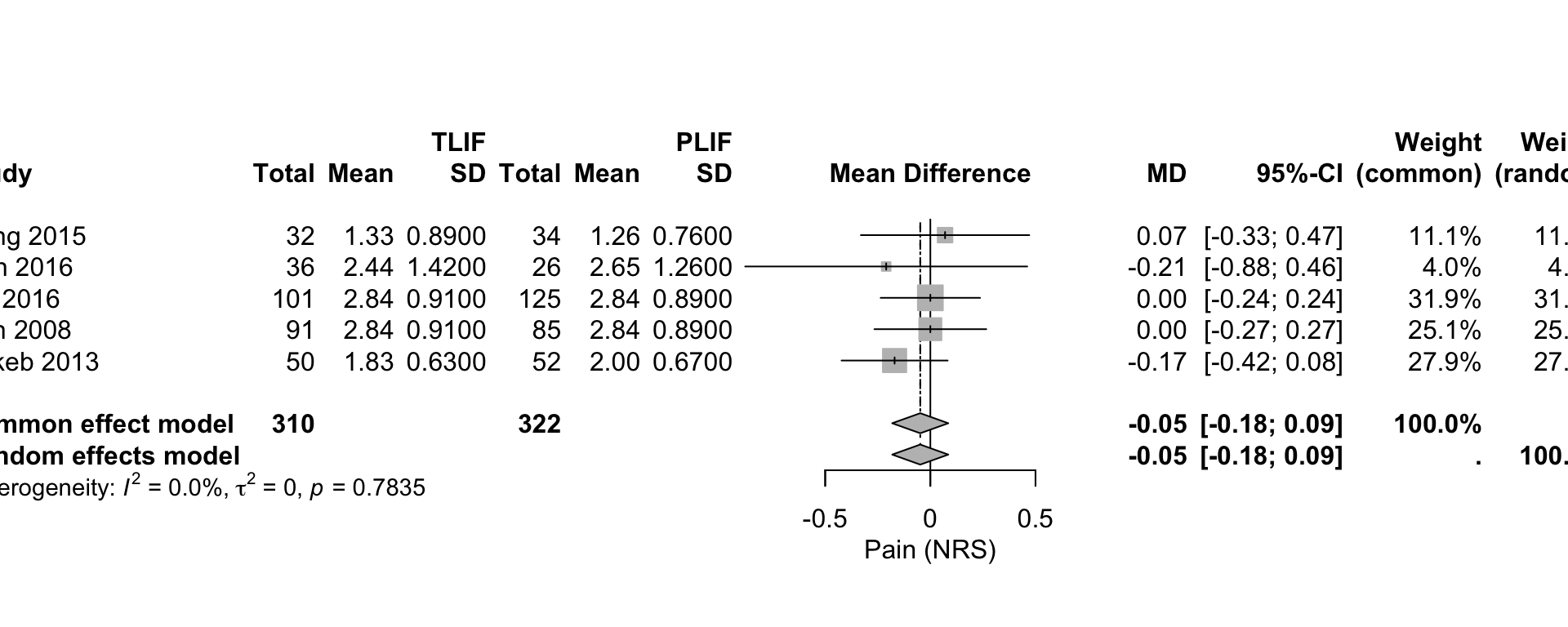
The pain scores hardly differ (MD −0.05, 95% CI −0.18 to 0.09) and there is no heterogeneity (I² = 0%).
Continuous outcomes: standardised mean difference
When studies measure the same outcome on different scales, use the standardised mean difference (SMD, Hedges’ g): the difference in means divided by the pooled standard deviation. Example: length of hospital stay after stroke in specialist versus routine care (dat.normand1999).
stroke <- escalc(measure = "SMD",
                 m1i = m1i, sd1i = sd1i, n1i = n1i,   # specialist care
                 m2i = m2i, sd2i = sd2i, n2i = n2i,   # routine care
                 data = dat.normand1999, slab = source)
res_smd <- rma(yi, vi, data = stroke)
print(res_smd, digits = 2)
Random-Effects Model (k = 9; tau^2 estimator: REML)

tau^2 (estimated amount of total heterogeneity): 0.79 (SE = 0.43)
tau (square root of estimated tau^2 value):      0.89
I^2 (total heterogeneity / total variability):   95.49%
H^2 (total variability / sampling variability):  22.20

Test for Heterogeneity:
Q(df = 8) = 123.73, p-val < .01

Model Results:

estimate    se   zval  pval  ci.lb  ci.ub
   -0.54  0.31  -1.74  0.08  -1.14   0.07  .

---
Signif. codes:  0 '***' 0.001 '**' 0.01 '*' 0.05 '.' 0.1 ' ' 1
The pooled SMD is −0.54 (95% CI −1.14 to 0.07): a moderate reduction in length of stay, but not statistically significant, and with very large heterogeneity (I² = 95%).
Saving a forest plot
To put a forest plot in your paper, save it as an image file. This is not run on the website.
png("forest_plot.png", width = 1000, height = 500)
forest(m_cont, label.e = "TLIF", label.c = "PLIF", xlab = "Pain (NRS)")
dev.off()
Check yourself
Go to the concept list and practice quiz of week 4 and try the practice quiz without looking at this page.