library(metafor)
library(metadat)
dat <- escalc(measure = "RR", ai = tpos, bi = tneg, ci = cpos, di = cneg,
              data = dat.bcg, slab = paste(author, year))
res <- rma(yi, vi, data = dat)R lecture 5: Heterogeneity and publication bias
SKI3011 · tau², I², prediction intervals, influence, cumulative meta-analysis, funnel plots
How to use this lecture. Download the R script, open it in RStudio and run it line by line (Cmd+Enter on a Mac, Ctrl+Enter on Windows). All explanations on this page are in the script as comments. Check that you get the same output as shown here. Quiz 4 asks you to read and interpret exactly this kind of code and output.
Packages and data
We start again with the BCG trials of lecture 3.
How much heterogeneity?
tau^2(τ²): the variance of the true effects between studies;tauis its square root.I^2: the share of the total variability due to real differences between studies rather than chance.H^2: total variability divided by sampling variability (1 means no heterogeneity).- The Q test: is there more variation than chance would explain? It has little power when there are few studies.
print(res, digits = 2)
Random-Effects Model (k = 13; tau^2 estimator: REML)

tau^2 (estimated amount of total heterogeneity): 0.31 (SE = 0.17)
tau (square root of estimated tau^2 value):      0.56
I^2 (total heterogeneity / total variability):   92.22%
H^2 (total variability / sampling variability):  12.86

Test for Heterogeneity:
Q(df = 12) = 152.23, p-val < .01

Model Results:

estimate    se   zval  pval  ci.lb  ci.ub
   -0.71  0.18  -3.97  <.01  -1.07  -0.36  ***

---
Signif. codes: 0 '***' 0.001 '**' 0.01 '*' 0.05 '.' 0.1 ' ' 1confint(res, digits = 2) # confidence intervals for tau^2 and I^2
       estimate ci.lb ci.ub
tau^2      0.31  0.12  1.11
tau        0.56  0.35  1.05
I^2(%)    92.22 81.92 97.68
H^2       12.86  5.53 43.07
I² is 92% (95% CI 82% to 98%): the effect of BCG differs strongly between trials.
The prediction interval
The confidence interval tells you how precisely the average effect is estimated. The prediction interval (pi.lb, pi.ub) tells you where the true effect of a new trial is expected to fall. With large τ² it is much wider.
predict(res, transf = exp, digits = 2)
 pred ci.lb ci.ub pi.lb pi.ub
 0.49  0.34  0.70  0.15  1.55
On average BCG halves the risk (RR 0.49), but in a new setting the effect could be anything from strong protection (0.15) to no protection or even harm (1.55).
Is one study driving the result?
leave1out() repeats the meta-analysis k times, each time without one study. If the pooled estimate or I² changes a lot when one study is left out, that study is influential.
leave1out(res, transf = exp, digits = 2)
                           estimate  zval pval ci.lb ci.ub      Q   Qp tau2
-Aronson 1948                  0.49 -3.72 0.00  0.34  0.72 151.58 0.00 0.34
-Ferguson & Simes 1949         0.52 -3.62 0.00  0.36  0.74 145.32 0.00 0.29
-Rosenthal et al 1960          0.50 -3.69 0.00  0.35  0.73 150.20 0.00 0.32
-Hart & Sutherland 1977        0.53 -3.56 0.00  0.38  0.75  96.56 0.00 0.26
-Frimodt-Moller et al 1973     0.47 -3.98 0.00  0.32  0.68 151.32 0.00 0.33
-Stein & Aronson 1953          0.49 -3.55 0.00  0.33  0.73 128.19 0.00 0.36
-Vandiviere et al 1973         0.52 -3.63 0.00  0.36  0.74 145.83 0.00 0.29
-TPT Madras 1980               0.45 -4.42 0.00  0.32  0.64  67.99 0.00 0.27
-Coetzee & Berjak 1968         0.48 -3.77 0.00  0.32  0.70 152.21 0.00 0.35
-Rosenthal et al 1961          0.52 -3.54 0.00  0.36  0.75 139.83 0.00 0.30
-Comstock et al 1974           0.47 -3.87 0.00  0.32  0.69 151.47 0.00 0.34
-Comstock & Webster 1969       0.47 -4.17 0.00  0.33  0.67 150.79 0.00 0.31
-Comstock et al 1976           0.46 -4.19 0.00  0.32  0.66 149.79 0.00 0.30
                              I2    H2
-Aronson 1948              93.23 14.76
-Ferguson & Simes 1949     92.25 12.91
-Rosenthal et al 1960      92.94 14.16
-Hart & Sutherland 1977    90.41 10.43
-Frimodt-Moller et al 1973 92.76 13.82
-Stein & Aronson 1953      90.91 11.00
-Vandiviere et al 1973     92.28 12.95
-TPT Madras 1980           87.03  7.71
-Coetzee & Berjak 1968     93.21 14.73
-Rosenthal et al 1961      92.23 12.87
-Comstock et al 1974       91.81 12.21
-Comstock & Webster 1969   92.68 13.66
-Comstock et al 1976       92.34 13.06
influence() gives formal diagnostics: studies marked with an asterisk are influential.
inf <- influence(res)
print(inf, digits = 2)
                          rstudent dffits cook.d cov.r tau2.del QE.del  hat
Aronson 1948                 -0.22  -0.04   0.00  1.12     0.34 151.58 0.05
Ferguson & Simes 1949        -1.29  -0.34   0.11  1.01     0.29 145.32 0.06
Rosenthal et al 1960         -0.75  -0.16   0.03  1.07     0.32 150.20 0.04
Hart & Sutherland 1977       -1.45  -0.52   0.23  0.97     0.26  96.56 0.10
Frimodt-Moller et al 1973     0.85   0.27   0.08  1.14     0.33 151.32 0.09
Stein & Aronson 1953         -0.12  -0.02   0.00  1.24     0.36 128.19 0.10
Vandiviere et al 1973        -1.30  -0.34   0.11  1.01     0.29 145.83 0.06
TPT Madras 1980               1.45   0.48   0.20  1.00     0.27  67.99 0.10
Coetzee & Berjak 1968         0.41   0.14   0.02  1.20     0.35 152.21 0.09
Rosenthal et al 1961         -1.13  -0.35   0.12  1.05     0.30 139.83 0.08
Comstock et al 1974           0.67   0.23   0.06  1.19     0.34 151.47 0.10
Comstock & Webster 1969       1.29   0.25   0.06  1.03     0.31 150.79 0.04
Comstock et al 1976           1.19   0.35   0.12  1.07     0.30 149.79 0.08
                          weight  dfbs inf
Aronson 1948                5.06 -0.04
Ferguson & Simes 1949       6.36 -0.35
Rosenthal et al 1960        4.44 -0.16
Hart & Sutherland 1977      9.70 -0.51
Frimodt-Moller et al 1973   8.87  0.27
Stein & Aronson 1953       10.10 -0.02
Vandiviere et al 1973       6.03 -0.34
TPT Madras 1980            10.19  0.47
Coetzee & Berjak 1968       8.74  0.14
Rosenthal et al 1961        8.37 -0.35
Comstock et al 1974         9.93  0.23
Comstock & Webster 1969     3.82  0.25
Comstock et al 1976 8.40 0.35 plot(inf)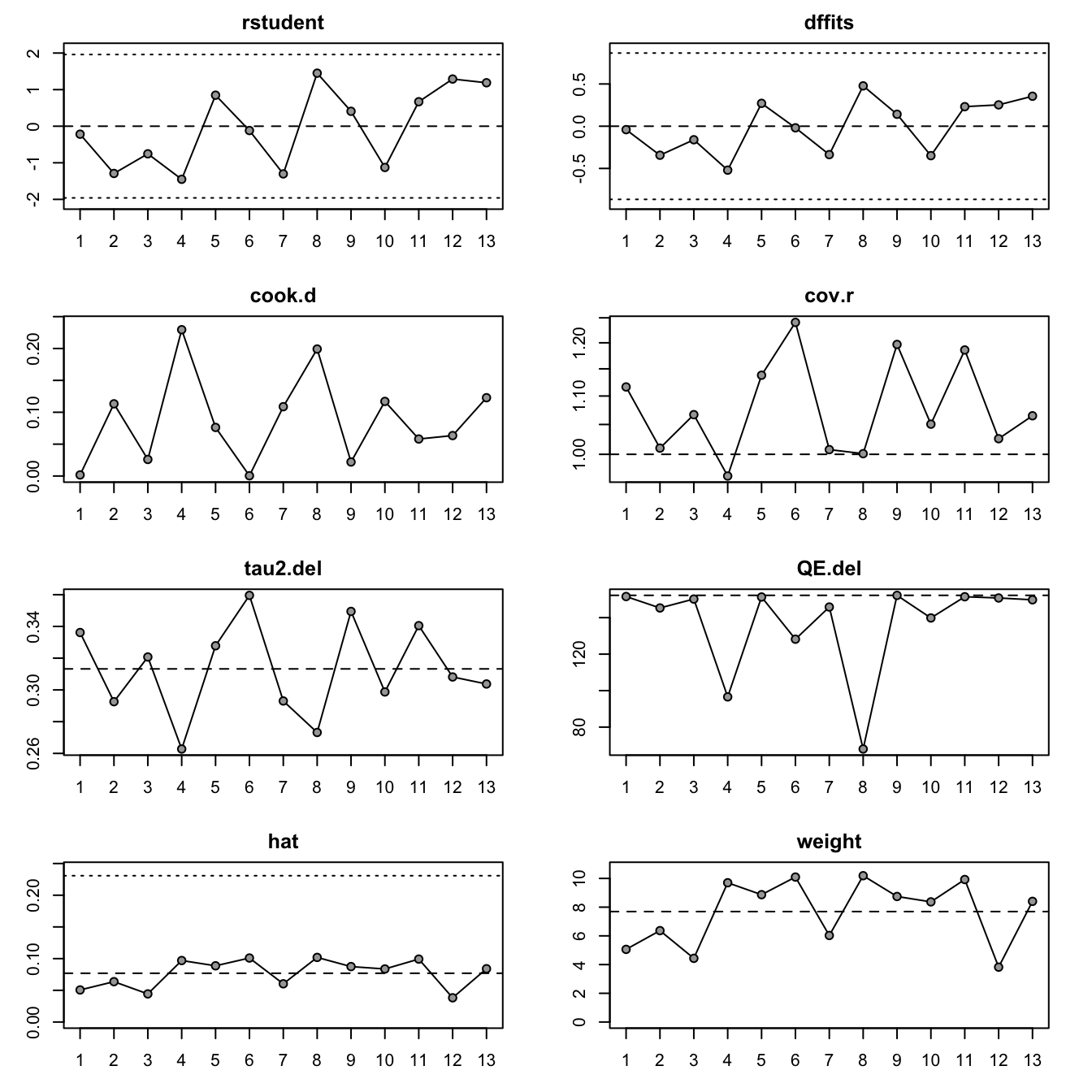
Cumulative meta-analysis
A cumulative meta-analysis adds the studies one by one, here in order of publication year. It shows how the evidence developed over time.
cum <- cumul(res, order = dat$year)
forest(cum, atransf = exp, header = TRUE)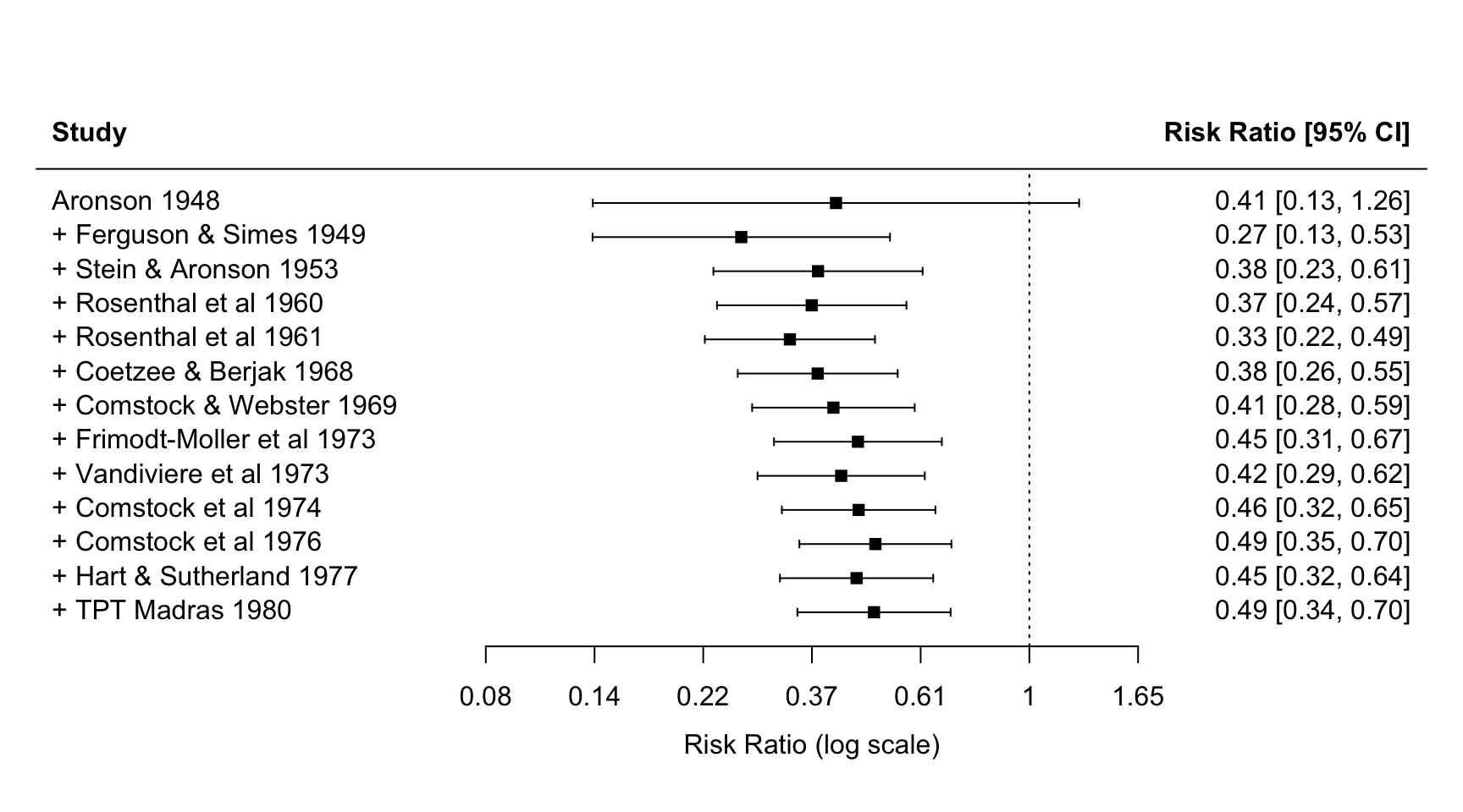
Publication bias: the magnesium story
16 trials of intravenous magnesium after a heart attack, outcome death (dat.egger2001). The small early trials suggested a large benefit. The last trial, ISIS-4 (1995), included more than 58,000 patients and found no benefit.
mag <- escalc(measure = "OR", ai = ai, n1i = n1i, ci = ci, n2i = n2i,
              data = dat.egger2001, slab = paste(study, year))
res_mag <- rma(yi, vi, data = mag)
predict(res_mag, transf = exp, digits = 2)
 pred ci.lb ci.ub pi.lb pi.ub
 0.46  0.31  0.70  0.15  1.45
The funnel plot
A funnel plot shows each study’s effect against its standard error. Without bias, small studies (at the bottom) scatter symmetrically around the pooled estimate. Here the small studies all sit on the side of a large benefit: the funnel is asymmetric.
funnel(res_mag, atransf = exp, xlab = "Odds ratio (log scale)")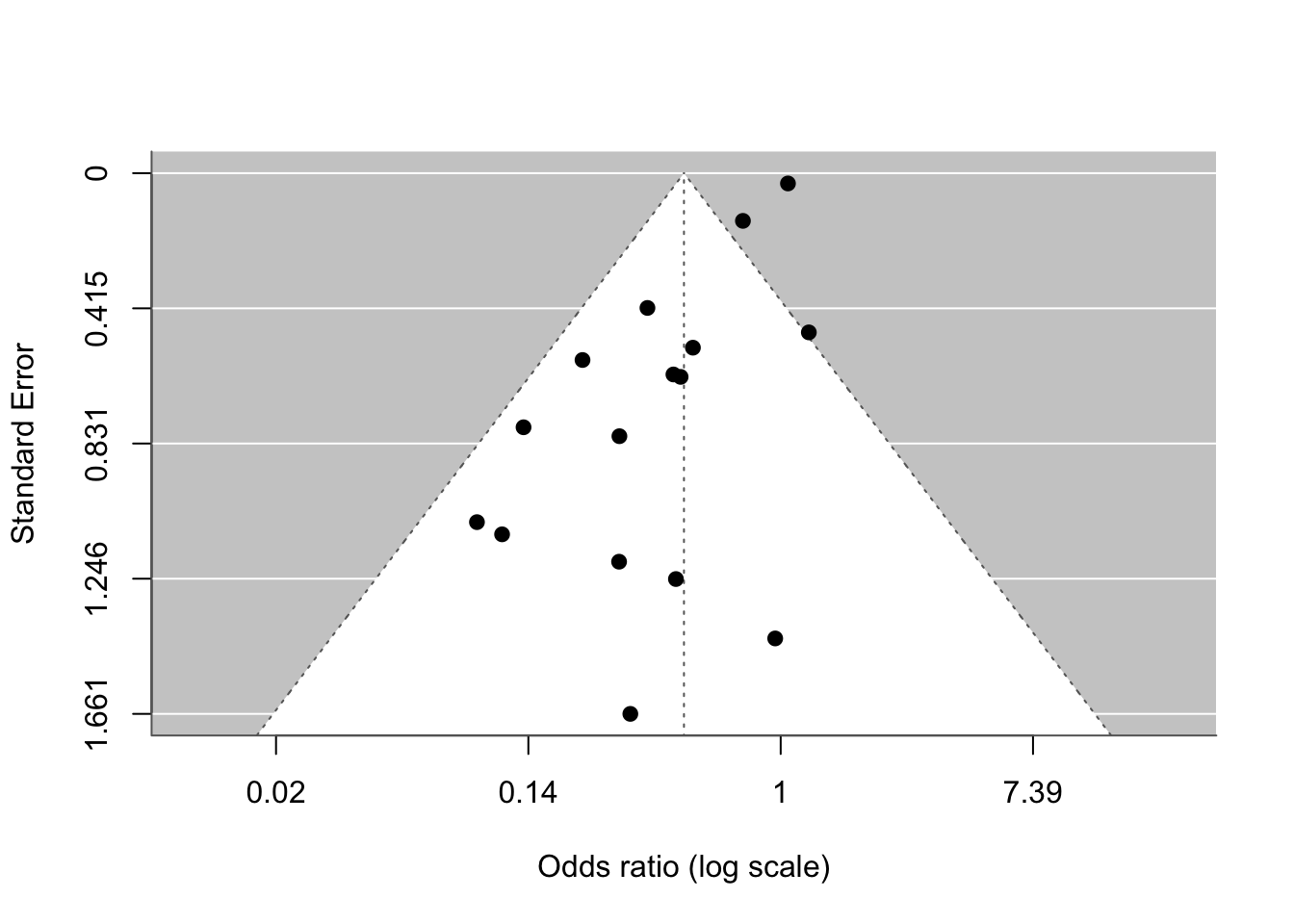
Egger’s test
regtest() tests funnel plot asymmetry. The limit estimate is the expected effect of an infinitely large study (standard error → 0).
regtest(res_mag)
Regression Test for Funnel Plot Asymmetry

Model:     mixed-effects meta-regression model
Predictor: standard error

Test for Funnel Plot Asymmetry: z = -4.6686, p < .0001
Limit Estimate (as sei -> 0):   b =  0.0419 (CI: -0.1604, 0.2443)
The test is clearly significant, and the limit estimate is close to 0 on the log scale (an OR of about 1): exactly what ISIS-4 found.
Trim-and-fill
trimfill() estimates how many studies are “missing” and what the pooled estimate would be if they were added. The filled studies appear as open circles in the funnel plot.
tf <- trimfill(res_mag)
predict(tf, transf = exp, digits = 2)
 pred ci.lb ci.ub pi.lb pi.ub
0.68 0.44 1.03 0.16 2.81 funnel(tf, atransf = exp, xlab = "Odds ratio (log scale)")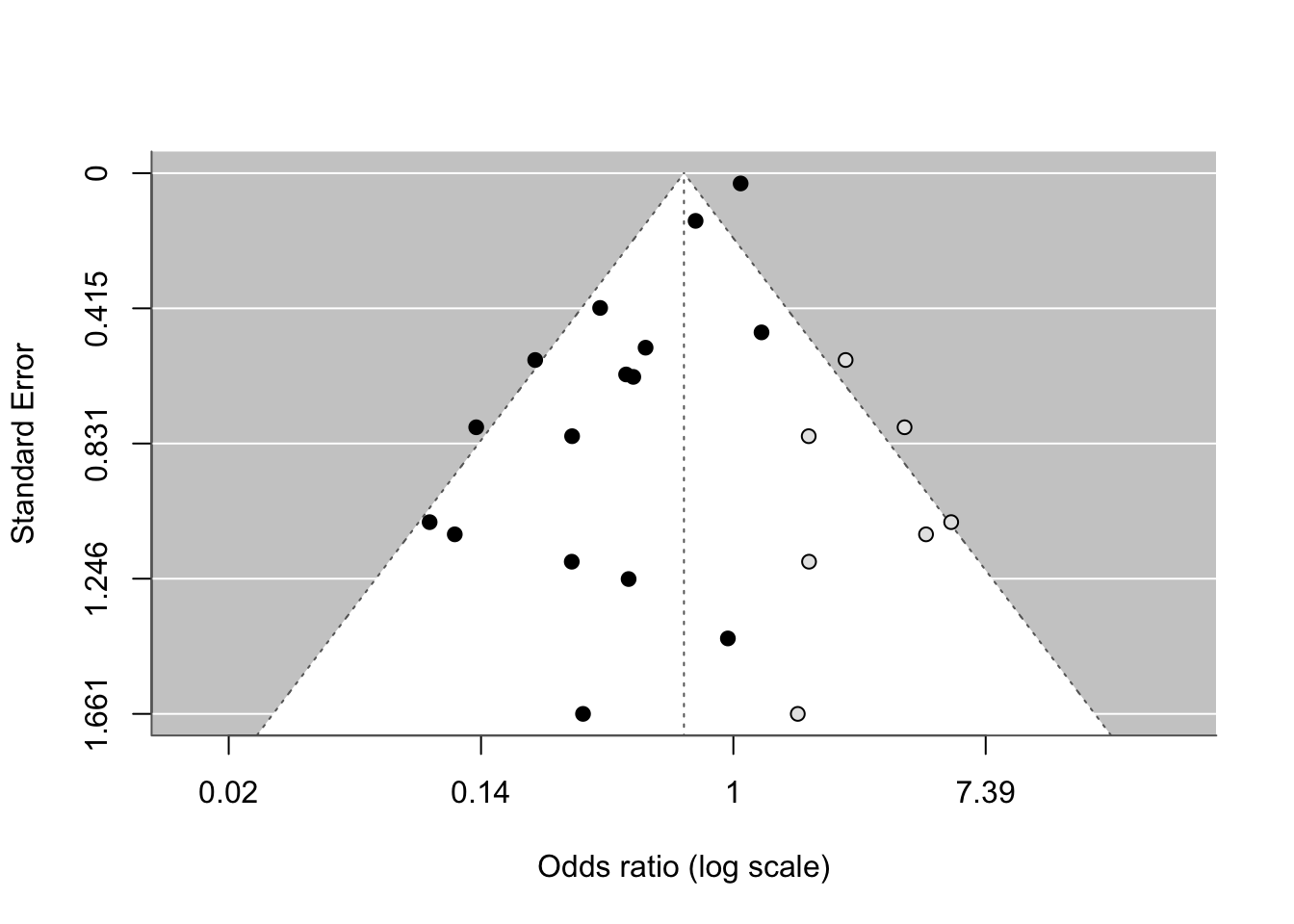
After filling 7 studies the OR rises from 0.46 to 0.68 and is no longer statistically significant. Trim-and-fill is a sensitivity analysis, not a correction: it shows how fragile the result is.
Small-study effects are not always publication bias
Funnel plot asymmetry means that small studies show different effects than large ones. Publication bias is one explanation; others are lower quality of small trials, different patients, or chance. With fewer than about 10 studies these tests have little power.
Check yourself
Go to the concept list and practice quiz of week 5 and try the practice quiz without looking at this page.