library(metafor)
library(metadat)
dat <- escalc(measure = "RR", ai = tpos, bi = tneg, ci = cpos, di = cneg,
data = dat.bcg, slab = paste(author, year))R lecture 6: Subgroup analysis and meta-regression
SKI3011 · categorical and continuous moderators, QM, QE, R²
How to use this lecture. Download the R script, open it in RStudio and run it line by line (Cmd+Enter on a Mac, Ctrl+Enter on Windows). All explanations on this page are in the script as comments. Check that you get the same output as shown here. Quiz 5 asks you to read and interpret exactly this kind of code and output.
Why subgroups and meta-regression?
Last week we saw large heterogeneity in the BCG trials. Can study characteristics (moderators) explain it? A subgroup analysis compares groups of studies; a meta-regression models the effect size as a function of a moderator. Both are observational: they compare studies, not patients.
Subgroups: separate meta-analyses
How were people allocated to vaccine or control? Randomly, alternately or systematically. First we pool each subgroup separately.
table(dat$alloc)
 alternate     random systematic
         2          7          4
res_random <- rma(yi, vi, data = dat, subset = alloc == "random")
res_alternate <- rma(yi, vi, data = dat, subset = alloc == "alternate")
res_systematic <- rma(yi, vi, data = dat, subset = alloc == "systematic")
predict(res_random, transf = exp, digits = 2)
 pred ci.lb ci.ub pi.lb pi.ub
0.38 0.22 0.65 0.10 1.45 predict(res_systematic, transf = exp, digits = 2)
 pred ci.lb ci.ub pi.lb pi.ub
 0.65  0.32  1.32  0.16  2.72
Subgroups: testing the difference
Do the subgroups really differ? Put the subgroup variable as a categorical moderator in the model with mods = ~ factor(...). QM (the test of moderators) tests whether the moderator explains heterogeneity; QE tests whether heterogeneity remains.
res_alloc <- rma(yi, vi, mods = ~ factor(alloc), data = dat)
print(res_alloc, digits = 2)
Mixed-Effects Model (k = 13; tau^2 estimator: REML)

tau^2 (estimated amount of residual heterogeneity):     0.36 (SE = 0.21)
tau (square root of estimated tau^2 value):             0.60
I^2 (residual heterogeneity / unaccounted variability): 88.77%
H^2 (unaccounted variability / sampling variability):   8.91
R^2 (amount of heterogeneity accounted for):            0.00%

Test for Residual Heterogeneity:
QE(df = 10) = 132.37, p-val < .01

Test of Moderators (coefficients 2:3):
QM(df = 2) = 1.77, p-val = 0.41

Model Results:

                         estimate    se   zval  pval  ci.lb  ci.ub
intrcpt                     -0.52  0.44  -1.17  0.24  -1.38   0.35
factor(alloc)random         -0.45  0.52  -0.87  0.39  -1.46   0.56
factor(alloc)systematic      0.09  0.56   0.16  0.87  -1.01   1.19

---
Signif. codes:  0 '***' 0.001 '**' 0.01 '*' 0.05 '.' 0.1 ' ' 1
The intercept is the reference group (alternate allocation); the other coefficients are differences from it. QM is not significant (p = 0.41) and R² is 0%: allocation method does not explain the heterogeneity.
A subgroup that does matter
Back to the 35 studies on loss of smell in COVID-19 patients of lecture 3. Studies that measured smell objectively (with a test) find more loss than studies that asked patients (subjective).
smell <- escalc(measure = "PR", xi = xi, ni = ni, data = dat.hannum2020)
table(smell$objectivity)
 Objective Subjective
         6         29
res_smell <- rma(yi, vi, mods = ~ objectivity, data = smell)
print(res_smell, digits = 2)
Mixed-Effects Model (k = 35; tau^2 estimator: REML)

tau^2 (estimated amount of residual heterogeneity):     0.05 (SE = 0.01)
tau (square root of estimated tau^2 value):             0.21
I^2 (residual heterogeneity / unaccounted variability): 99.07%
H^2 (unaccounted variability / sampling variability):   107.35
R^2 (amount of heterogeneity accounted for):            21.16%

Test for Residual Heterogeneity:
QE(df = 33) = 6524.64, p-val < .01

Test of Moderators (coefficient 2):
QM(df = 1) = 9.77, p-val < .01

Model Results:

                       estimate    se   zval  pval  ci.lb  ci.ub
intrcpt                    0.75  0.09   8.29  <.01   0.57   0.93  ***
objectivitySubjective     -0.31  0.10  -3.13  <.01  -0.50  -0.12   **

---
Signif. codes:  0 '***' 0.001 '**' 0.01 '*' 0.05 '.' 0.1 ' ' 1
Objective measurement: 75% of patients lose their sense of smell; subjective: 0.75 − 0.31 = 44%. The difference is significant (QM p < .01), but with 6 objective studies and still 99% residual heterogeneity.
Meta-regression with a continuous moderator
Absolute latitude (ablat): the distance of the trial site from the equator. One idea is that BCG works better far from the equator, where people are less exposed to other mycobacteria.
res_lat <- rma(yi, vi, mods = ~ ablat, data = dat)
print(res_lat, digits = 3)
Mixed-Effects Model (k = 13; tau^2 estimator: REML)

tau^2 (estimated amount of residual heterogeneity):     0.076 (SE = 0.059)
tau (square root of estimated tau^2 value):             0.276
I^2 (residual heterogeneity / unaccounted variability): 68.39%
H^2 (unaccounted variability / sampling variability):   3.16
R^2 (amount of heterogeneity accounted for):            75.62%

Test for Residual Heterogeneity:
QE(df = 11) = 30.733, p-val = 0.001

Test of Moderators (coefficient 2):
QM(df = 1) = 16.357, p-val < .001

Model Results:

         estimate     se    zval   pval   ci.lb   ci.ub
intrcpt     0.251  0.249   1.009  0.313  -0.237   0.740
ablat      -0.029  0.007  -4.044  <.001  -0.043  -0.015  ***

---
Signif. codes: 0 '***' 0.001 '**' 0.01 '*' 0.05 '.' 0.1 ' ' 1exp(coef(res_lat)["ablat"]) # change in the risk ratio per degree latitude ablat
0.9713177 Per degree further from the equator the RR is multiplied by 0.97. Latitude explains 76% of τ² (R²), but heterogeneity remains (QE p = 0.001).
The bubble plot
Each circle is a trial, sized by its weight; the line is the meta-regression.
regplot(res_lat, transf = exp, xlab = "Absolute latitude", ylab = "Risk ratio")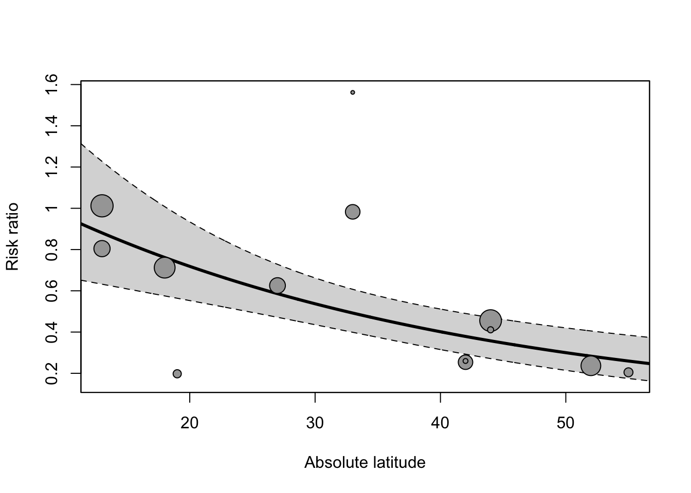
predict() with newmods gives the expected RR at chosen latitudes.
predict(res_lat, newmods = c(10, 30, 50), transf = exp, digits = 2)
  pred ci.lb ci.ub pi.lb pi.ub
1 0.96  0.67  1.39  0.50  1.85
2 0.54  0.44  0.66  0.30  0.96
3 0.30  0.21  0.42  0.16  0.57
More moderators: writing-to-learn
48 studies on writing-to-learn interventions in school (dat.bangertdrowns2004), outcome as standardised mean difference. Does a longer intervention work better? Does feedback help?
wtl <- dat.bangertdrowns2004
rma(yi, vi, mods = ~ length, data = wtl, digits = 3)            # length in weeks
Mixed-Effects Model (k = 46; tau^2 estimator: REML)

tau^2 (estimated amount of residual heterogeneity):     0.044 (SE = 0.019)
tau (square root of estimated tau^2 value):             0.210
I^2 (residual heterogeneity / unaccounted variability): 55.26%
H^2 (unaccounted variability / sampling variability):   2.24
R^2 (amount of heterogeneity accounted for):            5.08%

Test for Residual Heterogeneity:
QE(df = 44) = 96.281, p-val < .001

Test of Moderators (coefficient 2):
QM(df = 1) = 4.227, p-val = 0.040

Model Results:

         estimate     se   zval   pval   ci.lb  ci.ub
intrcpt     0.069  0.083  0.838  0.402  -0.093  0.231
length      0.015  0.007  2.056  0.040   0.001  0.029  *

---
Signif. codes: 0 '***' 0.001 '**' 0.01 '*' 0.05 '.' 0.1 ' ' 1rma(yi, vi, mods = ~ factor(feedback), data = wtl, digits = 2) # feedback yes/no
Mixed-Effects Model (k = 47; tau^2 estimator: REML)

tau^2 (estimated amount of residual heterogeneity):     0.05 (SE = 0.02)
tau (square root of estimated tau^2 value):             0.21
I^2 (residual heterogeneity / unaccounted variability): 55.81%
H^2 (unaccounted variability / sampling variability):   2.26
R^2 (amount of heterogeneity accounted for):            0.00%

Test for Residual Heterogeneity:
QE(df = 45) = 98.28, p-val < .01

Test of Moderators (coefficient 2):
QM(df = 1) = 0.94, p-val = 0.33

Model Results:

                   estimate    se  zval  pval  ci.lb  ci.ub
intrcpt                0.17  0.08  2.21  0.03   0.02   0.32  *
factor(feedback)1      0.09  0.10  0.97  0.33  -0.09   0.28

---
Signif. codes: 0 '***' 0.001 '**' 0.01 '*' 0.05 '.' 0.1 ' ' 1rma(yi, vi, mods = ~ length + factor(wic), data = wtl, digits = 3) # two moderators
Mixed-Effects Model (k = 44; tau^2 estimator: REML)

tau^2 (estimated amount of residual heterogeneity):     0.034 (SE = 0.017)
tau (square root of estimated tau^2 value):             0.185
I^2 (residual heterogeneity / unaccounted variability): 49.09%
H^2 (unaccounted variability / sampling variability):   1.96
R^2 (amount of heterogeneity accounted for):            0.00%

Test for Residual Heterogeneity:
QE(df = 41) = 79.943, p-val < .001

Test of Moderators (coefficients 2:3):
QM(df = 2) = 3.302, p-val = 0.192

Model Results:

              estimate     se    zval   pval   ci.lb  ci.ub
intrcpt          0.079  0.117   0.676  0.499  -0.150  0.309
length           0.012  0.007   1.793  0.073  -0.001  0.026  .
factor(wic)1    -0.005  0.103  -0.049  0.961  -0.207  0.197

---
Signif. codes:  0 '***' 0.001 '**' 0.01 '*' 0.05 '.' 0.1 ' ' 1
Each extra week adds 0.015 to the SMD (p = 0.04), but R² is only 5%. Feedback does not matter (p = 0.33). With two moderators the length effect is no longer significant. Note the message that studies with missing moderator values are left out.
Be careful with meta-regression
- About 10 studies per moderator: with fewer you have little power and unstable estimates.
- Plan moderators in your protocol: testing many moderators afterwards gives false positive findings.
- Moderators are often correlated with each other (confounding between study characteristics).
- Ecological fallacy: an association across studies (e.g. with mean age) does not prove the same association within individuals.
Check yourself
Go to the concept list and practice quiz of week 6 and try the practice quiz without looking at this page.